SWR StehwellenVerhältnis, ( Standig Wave Ratio)
Miroslav J. Dvorecky
Auf einer Hochfrequenz-Leitung die eine Quelle von elektromagnetischer Energie ( Oszillator etc.) mit einem Verbraucher ( z. B. Antenne ) verbindet, entstehen Stehende Wellen-Maxima und Wellen-Minima, falls die Impedanzen der Leitung und des Verbrauchers ungleich sind.
Die Lage und Grösse der Maxima und Minima lassen sich einfach messen.
Die energietransportierende Welle wird in diesem Fall am Ausgang der Leitung teilweise reflektiert und beginnt sich zurück zur Quelle zu bewegen. Die Amplituden der hinlaufenden und rücklaufenden Welle summieren sich und bilden Amplituden-Maxima und Minima (Knoten )
an eindeutigen Positionen der Leitung. Obwohl an einer bestimmten Position die Amplitude der Welle von Minus ins Plus schwingt, ändert sie ihre Lage nicht ( stehende Welle ).
U Amplitude der Spannung an der Stelle des Maximums, ( voltage of the standing wave
in maximum )
u Amplitude der Spannung an der Stelle des Minimums, ( voltage of the standing wave
in minimum )
S Stehwellenverhältnis, ( Standing Wave Ratio )
h Abstand der Minima, ( distance between the adjacent minima, a half of wavelength )
Z
Impedanz der Hochfrequenzleitung, Kabel, Hohlleiter, ( the impedance of the wave
guide, e.g. cable, tube )
z Impedanz angeschlossen am Ende der Leitung, ( terminating impedance on the end
of the wave guide )
P Leistung der hinlaufenden Welle, ( the power of the forward, incident wave )
p Leistung der rücklaufenden Welle, ( the power of the reflected wave )
r Spannungs-Reflexionskoefficient, ( voltage reflection coefficient )
d Rücklaufdämpfung, ( return loss )
R* Reflexionskoeffizient, ( reflection coefficient )
a Phasenwinkel eines Vektors, ( phase angle of a vector )
f Frequenz, ( frequency )
R Widerstand ( resistance )
X Imaginärteil eines Vektors, Reaktanz, ( reactance quantity of a vector )
1. S = U/u
2. r = ( S 1 ) / ( S + 1 )
3. d = 10 log ( P/p ) , Einheit / unity: dB ( deciBell )
4. d = 20 log r
Notiz / note:
d = 10 log ( P/p )
d/10 = log ( P/p )
P/p = 10 exp( d/10 )
[ zehn hoch (d/10) ]
[ ten powered by (d/10) ]
5. R* = ( z Z ) / ( z + Z )
Impedanz ist eine komplexe Zahl ( Vektor ), und deswegen ist R* auch ein Vektor:
R* = |R*| ( cos a + j sin a ) = R* + j X*
Z = R + j X
( Z and z are complex quantities and therefor is R* also a vector )
6. 300 / 2 h = f [ meter, MHz ]
Beispiel / example
Auf einer Leitung wurde Stehwellenverhältnis S = 1,5 gemessen.
( On a wave guide was measured the SWR: S = 1.5 ).
Impedanz der Leitung beträgt 50 Ohm.
( Given, the line impedance Z is 50 Ohm ).
Z = 50 Ohm
r = ( S 1 ) / ( S + 1 ) = ( 1.5 1 ) / ( 1.5 + 1 ) = 0.2
d = 20 log r = 20 log 0.2 = 13.979 dB
P/p = 10 exp (d/10) = 10 exp ( 13.979 / 10 ) = 24.998
p = P / 24.998 Rücklaufleistung ( reflected power from load )
Gegeben / given P = 100 mW
Im Verbraucher nutzbare Leistung ist: 100 mW ( 100 / 24.998 ) = 100 4 = 96 mW
( Effective exciting power in load is 96 miliwatt, reflected power is 4 mW ).
Das bedeutet dass die Impedanz der Belastung von der Impedanz der Leitung abweicht.
( That means, that the load does not match the impedance of the feeding line ).
Nehmen wir an, dass die reale Komponenten der Impedanzen wesentlich grösser als die
Blindkomponenten X sind.
( Assume, that the real quantities of the impedances are much greater than the reactive quantities X ).
Unter dieser Bedingung gilt:
( Under this condition we can write ):
|R*| = r = 0.2 ( Absolute value of R*, the phase of the vector is ignored )
|R*| = ( z Z ) / ( z + Z ) = ( z 50 ) / ( z + 50 ) = 0.2
z 50 = 0.2 ( z + 50 ) = 0.2 z + 10
z 0.2 z = 10 + 50 = 60
0.8 z = 60
z = 60 / 0.8 = 75 Ohm Load impedance
h = 0.1 [ m] Gemessene Entfernung zwischen benachbarten Minima ( Knoten ) in Metern
( Measured distance between adjacent nodes - minima - in meter unit )
f = 300 / 2 ( 0.1 ) = 300 / 0.2 = 1 500 MHz = 1.5 GHz
Diese Berechnung ist nicht ganz genau, weil die elektromagnetische Welle sich in dem Wellenleiter
um ca. 5 % landsamer bewegt als im Vacuum. Für sie scheint die Leitung länger zu sein.
This calculation is not exact, due to slower propagation of the electro-magnetic wave in the
wave guide relating to its velocity in vacuum. It "sees" the wave guide longer by ca. 5 %.
Bestimmung des Last-Impedanzcharakters, ( determination of property of the load impedance ).
Die Belastungsimpedanz wird durch einen Kurzschluss ersetzt. Die Lage eines Minimums wird notiert.
Danach wird die Leitung mit der Belastungsimpedanz abgeschlossen. Jetzt befindet sich das
Minimum an anderer Stelle. Ist diese Stelle in der Richtung zur Belastungsimpedanz
verschoben, dann hat die reaktive Komponente der Belastungsimpedanz kapazitiven charakter.
Die Richtung zum Generator gibt induktiven Charakter an.
Gemessen werden immer nur benachbarte Minima und Maxima, weil entlang der Leitung ihre
Grösse nach bestimmter hyperbolischen Sinusfunktion verlaufen. Das Verhältnis bleibt dabei
aber konstant.
( Replace the load with a short. Note the position of any minimum-node.
Repeat the measurig with the load.
If the new position of minimum is displaced towards the load, than the impedance of load has capacitive character.
Shift of the minimum towards the generator indicates inductive character.
Only neighbourly positioned minima and maxima will be measured, because the voltage value of them
follows a hyperbolical sine function along the line, but the ratio of the voltage remains constant. )
TABELLE
SWR Voltage reflection coefficient Power reflected Return loss
( S ) ( r ) ( p ) % ( d ) dB
1.0 0 0 0
1.1 0.0476 0.227 26.44
1.2 0.0909 0.82 20.827
1.3 0.13 1.702 17.69
1.4 0.166 2.797 15.56
1.5 0.2 4.000 13.979
1.6 0.230 5.326 12.736
1.7 0.259 6,722 11.725
1.8 0.286 8.164 10.881
1.9 0.310 9.632 10.163
2.0 0.333 11.112 9.542
2.1 0.355 12.591 8.999
2.2 0.375 14.062 8.519
2.3 0.394 15.518 8.091
2.4 0.411 16.955 7.707
2.5 0,428 18.318 7.371
3.0 0.5 25.000 6.020
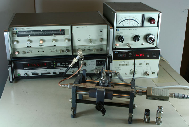
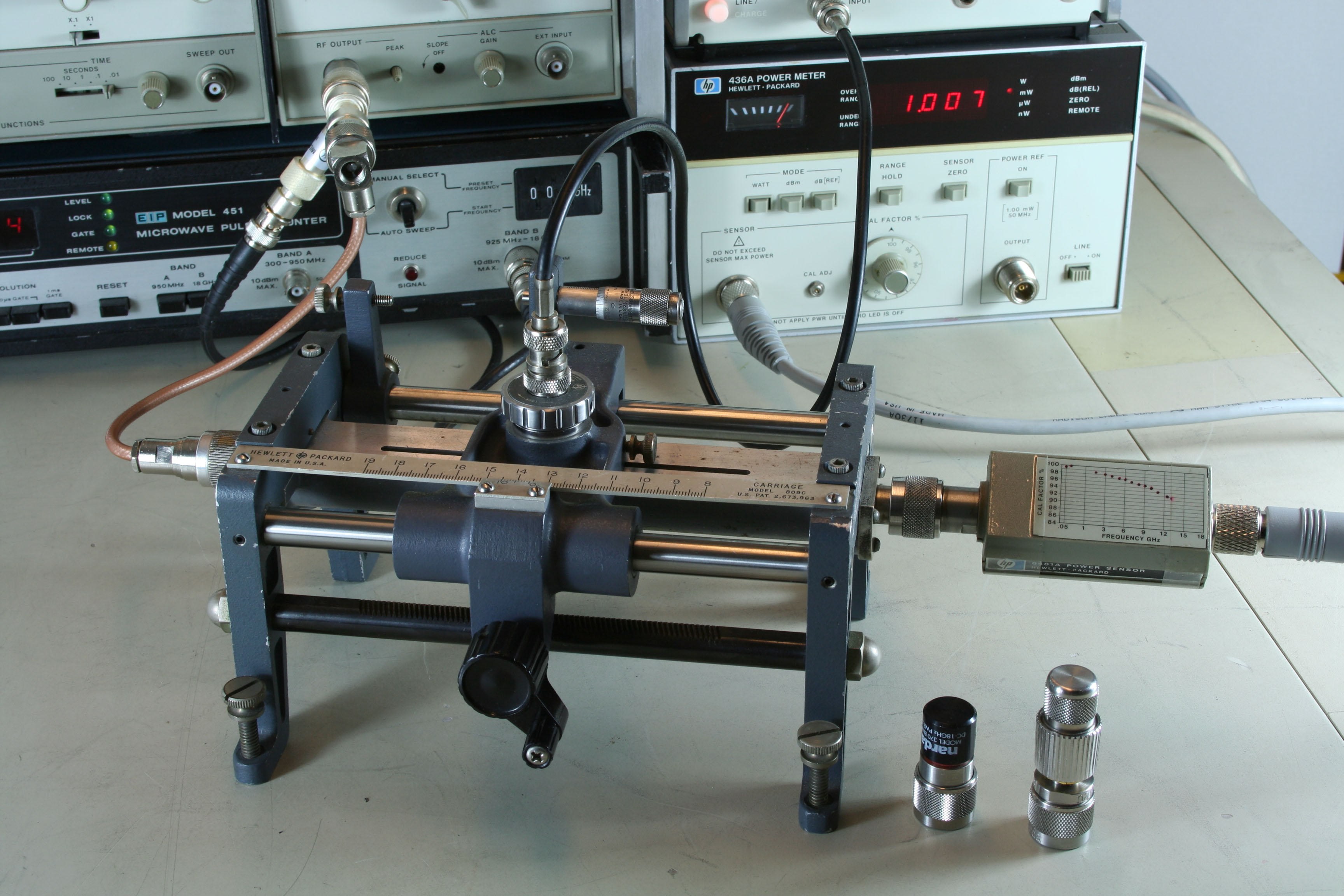
Der Messaufbau für Messung des SWR eines Leistungs-Sensors im Frequenzbereich bis 18 GHz
ist an folgenden Bildern sichtbar.
Das Signal ( 13.555 GHz ) ist mit 1 kHz moduliert, und durch die geschlitzte Messleitung zum Leistugs - Sensor geführt, dessen Reflexionsfaktor zu bestimmen ist.
Die Sonde der geschlitzten Messleitung demoduliert das Signal der stehenden Welle und führt
es zum SWR direktmessendem Voltmeter hp 415E. Ein koaxialer Kurzschluss und ein
koaxialer Abschlusswiderstand 50 Ohm sind unten rechts abgebildet.
( On following photographs is illustrated an Test Set Up For Slotted Line Measurement.
The signal modulated with 1 kHz from generator hp 8620C is fed throu the slotted line
hp 809C to an DUT - Device Under Test - which is a power sensor. The detected SWR signal
from the crystal diode probe is evaluated in voltmeter hp 415E, which scale is
calibrated direct in SWR. A dummy load 50 Ohm and a short lies at the output of the slotted line.)
Copyright Delektron Datensysteme T.u.H. GmbH 2008, München Germany
Copyright Delektron Datensysteme T.u.H. GmbH 2008, München Germany